# ruff: noqa: E402
# ruff: noqa: E501

Fitting a polynomial with Gaussian priors

We fit a simple polynomial with Gaussian priors, which is an example of a Gauss-linear problem.

import itertools

import numpy as np
import pandas as pd

np.set_printoptions(suppress=True)
rng = np.random.default_rng(12345)

import matplotlib.pyplot as plt

COLORS = list(plt.rcParams["axes.prop_cycle"].by_key()["color"])

plt.rcParams["figure.figsize"] = (6, 6)
plt.rcParams.update({"font.size": 10})
from ipywidgets import interact  # noqa  # isort:skip
import ipywidgets as widgets  # noqa  # isort:skip
from p_tqdm import p_map

import iterative_ensemble_smoother as ies

Define synthetic truth and use it to create noisy observations

ensemble_size = 200


def poly(a, b, c, x):
    return a * x**2 + b * x + c


# True parameter values
a_t = 0.5
b_t = 1.0
c_t = 3.0

noise_scale = 0.1
x_observations = [0, 2, 4, 6, 8]
observations = [
    (
        rng.normal(loc=1, scale=noise_scale) * poly(a_t, b_t, c_t, x),
        noise_scale * poly(a_t, b_t, c_t, x),
        x,
    )
    for x in x_observations
]

d = pd.DataFrame(observations, columns=["value", "sd", "x"])
d = d.set_index("x")
num_obs = d.shape[0]

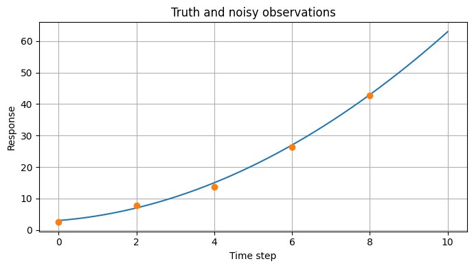
fig, ax = plt.subplots(figsize=(7, 4))
x_plot = np.linspace(0, 10, 2**8)
ax.set_title("Truth and noisy observations")
ax.set_xlabel("Time step")
ax.set_ylabel("Response")
ax.plot(x_plot, poly(a_t, b_t, c_t, x_plot))
ax.plot(d.index.get_level_values("x"), d.value.values, "o")
ax.grid()
fig.tight_layout()
plt.show()

Assume diagonal observation error covariance matrix and define perturbed observations

R = np.diag(d.sd.to_numpy() ** 2)

E = rng.multivariate_normal(mean=np.zeros(len(R)), cov=R, size=ensemble_size).T
assert E.shape == (num_obs, ensemble_size)

D = d.value.to_numpy().reshape(-1, 1) + E

Define Gaussian priors

coeff_a = rng.standard_normal(size=ensemble_size)
coeff_b = rng.standard_normal(size=ensemble_size)
coeff_c = rng.standard_normal(size=ensemble_size)

X = np.vstack([coeff_a, coeff_b, coeff_c])

Run forward model in parallel

fwd_runs = p_map(
    poly,
    coeff_a,
    coeff_b,
    coeff_c,
    [np.arange(max(x_observations) + 1)] * ensemble_size,
    desc="Running forward model.",
)

Pick responses where we have observations

Y = np.array(
    [fwd_run[d.index.get_level_values("x").to_list()] for fwd_run in fwd_runs]
).T

assert Y.shape == (
    num_obs,
    ensemble_size,
), (
    "Measured responses must be a matrix with dimensions (number of observations x number of realisations)"
)

Condition on observations to calculate posterior using both ESMDA

X_ESMDA = X.copy()
Y_ESMDA = Y.copy()
smoother = ies.ESMDA(
    covariance=d.sd.to_numpy() ** 2,
    observations=d.value.to_numpy(),
    seed=42,
)

for _ in range(smoother.num_assimilations()):
    # Assimilation step
    smoother.prepare_assimilation(Y=Y_ESMDA, truncation=1.0)
    X_ESMDA = smoother.assimilate_batch(X=X_ESMDA)

    # Apply forward model again
    _coeff_a, _coeff_b, _coeff_c = X_ESMDA
    x = [np.arange(max(x_observations) + 1)] * ensemble_size
    _fwd_runs = [
        poly(_coeff_a[i], _coeff_b[i], _coeff_c[i], x[i]) for i in range(len(_coeff_a))
    ]
    Y_ESMDA = np.array(
        [fwd_run[d.index.get_level_values("x").to_list()] for fwd_run in _fwd_runs]
    ).T

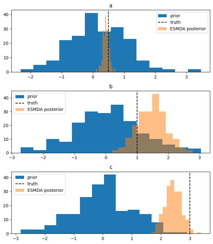
Plots to compare results

def plot_posterior(ax, posterior, method):
    for i, param in enumerate("abc"):
        ax[i].set_title(param)
        ax[i].hist(posterior[i, :], label=f"{method} posterior", alpha=0.5, bins="fd")
        ax[i].legend()

    fig.tight_layout()
    return ax


fig, ax = plt.subplots(nrows=3, figsize=(7, 8))

for i in range(3):
    ax[i].hist(X[i, :], label="prior", bins="fd")

ax[0].axvline(a_t, color="k", linestyle="--", label="truth")
ax[1].axvline(b_t, color="k", linestyle="--", label="truth")
ax[2].axvline(c_t, color="k", linestyle="--", label="truth")

plot_posterior(ax, X_ESMDA, method="ESMDA")

array([<Axes: title={'center': 'a'}>, <Axes: title={'center': 'b'}>,
       <Axes: title={'center': 'c'}>], dtype=object)

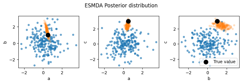
fig, axes = plt.subplots(1, 3, figsize=(8, 2.75))
axes = axes.ravel()
labels = "abc"
true_parameters = [a_t, b_t, c_t]

fig.suptitle("ESMDA Posterior distribution")
for k, (i, j) in enumerate(itertools.combinations([0, 1, 2], 2)):
    axes[k].scatter(X[i, :], X[j, :], s=15, alpha=0.6)
    axes[k].scatter(X_ESMDA[i, :], X_ESMDA[j, :], s=15, alpha=0.2)
    axes[k].scatter(
        [true_parameters[i]],
        [true_parameters[j]],
        color="black",
        s=100,
        label="True value",
    )
    axes[k].set_xlabel(labels[i])
    axes[k].set_ylabel(labels[j])


axes[k].legend()
fig.tight_layout()
plt.show()

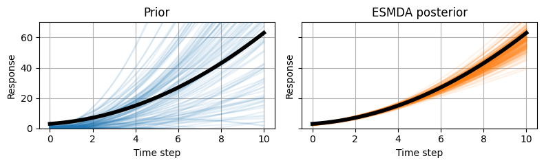
fig, (ax1, ax2) = plt.subplots(1, 2, figsize=(8, 2.5), sharex=True, sharey=True)
x_plot = np.linspace(0, 10, 2**8)

# Plot the prior
ax1.set_title("Prior")
ax1.plot(x_plot, poly(a_t, b_t, c_t, x_plot), zorder=10, lw=4, color="black")
for parameter_prior in X.T:
    ax1.plot(
        x_plot, poly(*parameter_prior, x_plot), color=COLORS[0], alpha=0.1, zorder=5
    )

# Plot the posterior
ax2.set_title("ESMDA posterior")
ax2.plot(x_plot, poly(a_t, b_t, c_t, x_plot), zorder=10, lw=4, color="black")
for parameter_posterior in X_ESMDA.T:
    ax2.plot(
        x_plot, poly(*parameter_posterior, x_plot), alpha=0.1, zorder=5, color=COLORS[1]
    )


# Common axes setup
for ax in [ax1, ax2]:
    ax.set_ylim([0, 70])
    ax.set_xlabel("Time step")
    ax.set_ylabel("Response")
    ax.grid(zorder=0)

fig.tight_layout()
plt.show()