# ruff: noqa: E402

Linear regression with ESMDA

We solve a linear regression problem using ESMDA. First we define the forward model as \(g(x) = Ax\), then we set up a prior ensemble on the linear regression coefficients, so \(x \sim \mathcal{N}(0, 1)\).

As shown in the 2013 paper by Emerick et al, when a set of inflation weights \(\alpha_i\) is chosen so that \(\sum_i \alpha_i^{-1} = 1\), ESMDA yields the correct posterior mean for the linear-Gaussian case.

Import packages

import numpy as np
from matplotlib import pyplot as plt

from iterative_ensemble_smoother import ESMDA

Create problem data

Some settings worth experimenting with:

• Decreasing prior_std=1 will pull the posterior solution toward zero.

• Increasing num_ensemble will increase the quality of the solution.

• Increasing num_observations / num_parameters will increase the quality of the solution.

num_parameters = 25
num_observations = 100
num_ensemble = 30
prior_std = 1

rng = np.random.default_rng(42)

# Create a problem with g(x) = A @ x
A = rng.standard_normal(size=(num_observations, num_parameters))


def g(X):
    """Forward model."""
    return A @ X


# Create observations: obs = g(x) + N(0, 1)
x_true = np.linspace(-1, 1, num=num_parameters)
observation_noise = rng.standard_normal(size=num_observations)
observations = g(x_true) + observation_noise

# Initial ensemble X ~ N(0, prior_std) and diagonal covariance with ones
X = rng.normal(size=(num_parameters, num_ensemble)) * prior_std

# Covariance matches the noise added to observations above
covariance = np.ones(num_observations)

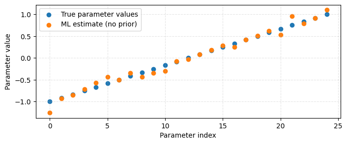
Solve the maximum likelihood problem

We can solve \(Ax = b\), where \(b\) is the observations, for the maximum likelihood estimate. Notice that unlike using a Ridge model, solving \(Ax = b\) directly does not use any prior information.

x_ml, *_ = np.linalg.lstsq(A, observations, rcond=None)

plt.figure(figsize=(8, 3))
plt.scatter(np.arange(len(x_true)), x_true, label="True parameter values")
plt.scatter(np.arange(len(x_true)), x_ml, label="ML estimate (no prior)")
plt.xlabel("Parameter index")
plt.ylabel("Parameter value")
plt.grid(True, ls="--", zorder=0, alpha=0.33)
plt.legend()
plt.show()

Solve using ESMDA

We crease an ESMDA instance and solve the Guass-linear problem.

smoother = ESMDA(
    covariance=covariance,
    observations=observations,
    alpha=5,
    seed=1,
)

X_i = np.copy(X)
for i, alpha_i in enumerate(smoother.alpha, 1):
    print(
        f"ESMDA iteration {i}/{smoother.num_assimilations()}"
        f" with inflation factor alpha_i={alpha_i}"
    )
    smoother.prepare_assimilation(Y=g(X_i))
    X_i = smoother.assimilate_batch(X=X_i)


X_posterior = np.copy(X_i)

ESMDA iteration 1/5 with inflation factor alpha_i=5.0
ESMDA iteration 2/5 with inflation factor alpha_i=5.0
ESMDA iteration 3/5 with inflation factor alpha_i=5.0
ESMDA iteration 4/5 with inflation factor alpha_i=5.0
ESMDA iteration 5/5 with inflation factor alpha_i=5.0

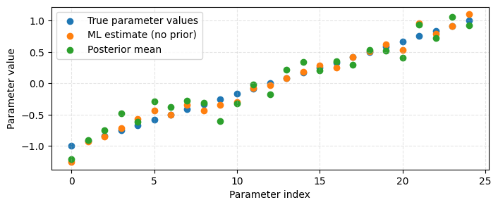
Plot and compare solutions

Compare the true parameters with both the ML estimate from linear regression and the posterior means obtained using ESMDA.

plt.figure(figsize=(8, 3))
plt.scatter(np.arange(len(x_true)), x_true, label="True parameter values")
plt.scatter(np.arange(len(x_true)), x_ml, label="ML estimate (no prior)")
plt.scatter(
    np.arange(len(x_true)), np.mean(X_posterior, axis=1), label="Posterior mean"
)
plt.xlabel("Parameter index")
plt.ylabel("Parameter value")
plt.grid(True, ls="--", zorder=0, alpha=0.33)
plt.legend()
plt.show()

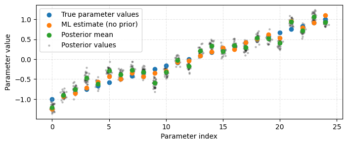
We now include the posterior samples as well.

plt.figure(figsize=(8, 3))
plt.scatter(np.arange(len(x_true)), x_true, label="True parameter values")
plt.scatter(np.arange(len(x_true)), x_ml, label="ML estimate (no prior)")
plt.scatter(
    np.arange(len(x_true)), np.mean(X_posterior, axis=1), label="Posterior mean"
)

# Loop over every ensemble member and plot it
for j in range(num_ensemble):
    # Jitter along the x-axis a little bit
    x_jitter = np.arange(len(x_true)) + rng.normal(loc=0, scale=0.1, size=len(x_true))

    # Plot this ensemble member
    plt.scatter(
        x_jitter,
        X_posterior[:, j],
        label=("Posterior values" if j == 0 else None),
        color="black",
        alpha=0.2,
        s=5,
        zorder=0,
    )
plt.xlabel("Parameter index")
plt.ylabel("Parameter value")
plt.grid(True, ls="--", zorder=0, alpha=0.33)
plt.legend()
plt.show()