# ruff: noqa: E402

Adaptive Localization

In this example we run adaptive localization on a sparse Gauss-linear problem.

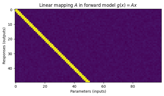
• Each response is only affected by \(3\) parameters.

• This is represented by a tridiagonal matrix \(A\) in the forward model \(g(x) = Ax\).

• The problem is Gauss-Linear, so in this case ESMDA will sample the true posterior when the number of ensemble members (realizations) is large.

• The sparse correlation structure will lead to spurious correlations, in the sense that a parameter and response might appear correlated when in fact they are not.

Import packages

import numpy as np
import scipy as sp
from matplotlib import pyplot as plt

from iterative_ensemble_smoother import ESMDA, AdaptiveESMDA

Create problem data

Some settings worth experimenting with:

• Decreasing prior_std=1 will pull the posterior solution toward zero.

• Increasing num_ensemble will increase the quality of the solution.

• Increasing num_observations / num_parameters will increase the quality of the solution.

rng = np.random.default_rng(42)

# Dimensionality of the problem
num_parameters = 100
num_observations = 50
num_ensemble = 25
prior_std = 1

# Number of iterations to use in ESMDA
alpha = 5

Create problem data - sparse tridiagonal matrix \(A\)

diagonal = np.ones(min(num_parameters, num_observations))

# Create a tridiagonal matrix (easiest with scipy)
A = sp.sparse.diags(
    [diagonal, diagonal, diagonal],
    offsets=[-1, 0, 1],
    shape=(num_observations, num_parameters),
    dtype=float,
).toarray()

# We add some noise that is insignificant compared to the
# actual local structure in the forward model
A = A + rng.standard_normal(size=A.shape) * 0.01

plt.title("Linear mapping $A$ in forward model $g(x) = Ax$")
plt.imshow(A)
plt.xlabel("Parameters (inputs)")
plt.ylabel("Responses (outputs)")
plt.tight_layout()
plt.show()

• Below we draw prior realizations \(X \sim N(0, \sigma)\).

• The true parameter values used to generate observations are in the range \([-1, 1]\).

• As the number of realizations (ensemble members) goes to infinity, the correlation between the prior and the true parameter values converges to zero.

• The correlation is zero for a finite number of realizations too, but statistical noise might induce some spurious correlations between the prior and the true parameter values.

In summary the baseline correlation is zero. Anything we can do to increase the correlation above zero beats the baseline, which is using the prior (no update).

The correlation coefficient does not take into account the uncertainty represented in the posterior, only the mean posterior value is compared with the true parameter values. To compare distributions we could use the Kullback–Leibler divergence, but we do not pursue this here.

def get_prior(num_parameters, num_ensemble, prior_std):
    """Sample prior from N(0, prior_std)."""
    return rng.normal(size=(num_parameters, num_ensemble)) * prior_std


def g(X):
    """Apply the forward model."""
    return A @ X


# Create observations: obs = g(x) + N(0, 1)
x_true = np.linspace(-1, 1, num=num_parameters)
observation_noise = rng.standard_normal(size=num_observations)  # N(0, 1) noise
observations = g(x_true) + observation_noise

# Initial ensemble X ~ N(0, prior_std) and diagonal covariance with ones
X = get_prior(num_parameters, num_ensemble, prior_std)

# Covariance matches the noise added to observations above
covariance = np.ones(num_observations)  # N(0, 1) covariance

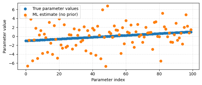
Solve the maximum likelihood problem

We can solve \(Ax = b\), where \(b\) are the observations, for the maximum likelihood estimate.

Notice that unlike using a Ridge model, solving \(Ax = b\) directly does not use any prior information.

x_ml, *_ = np.linalg.lstsq(A, observations, rcond=None)

plt.figure(figsize=(7, 3))
plt.scatter(np.arange(len(x_true)), x_true, label="True parameter values")
plt.scatter(np.arange(len(x_true)), x_ml, label="ML estimate (no prior)")
plt.xlabel("Parameter index")
plt.ylabel("Parameter value")
plt.grid(True, ls="--", zorder=0, alpha=0.33)
plt.legend()
plt.tight_layout()
plt.show()

Solve using ESMDA

We create an ESMDA instance and solve the Guass-linear problem.

smoother = ESMDA(
    covariance=covariance,
    observations=observations,
    alpha=alpha,
    seed=1,
)

X_i = np.copy(X)
for i in range(smoother.num_assimilations()):
    print(f"ESMDA iteration {i + 1}/{smoother.num_assimilations()}")
    smoother.prepare_assimilation(Y=g(X_i))
    X_i = smoother.assimilate_batch(X=X_i)


X_posterior = np.copy(X_i)

ESMDA iteration 1/5
ESMDA iteration 2/5
ESMDA iteration 3/5
ESMDA iteration 4/5
ESMDA iteration 5/5

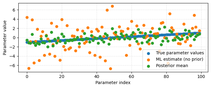
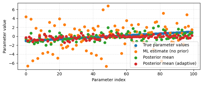
Plot and compare solutions

Compare the true parameters with both the ML estimate from linear regression and the posterior means obtained using ESMDA.

plt.figure(figsize=(7, 3))
plt.scatter(np.arange(len(x_true)), x_true, label="True parameter values")
plt.scatter(np.arange(len(x_true)), x_ml, label="ML estimate (no prior)")
plt.scatter(
    np.arange(len(x_true)), np.mean(X_posterior, axis=1), label="Posterior mean"
)
plt.xlabel("Parameter index")
plt.ylabel("Parameter value")
plt.grid(True, ls="--", zorder=0, alpha=0.33)
plt.legend()
plt.tight_layout()
plt.show()

Solve using AdaptiveESMDA

We create an AdaptiveESMDA instance and solve the Guass-linear problem.

adaptive_smoother = AdaptiveESMDA(
    covariance=covariance, observations=observations, seed=1, alpha=alpha
)

X_i = np.copy(X)


num_assimilations = adaptive_smoother.num_assimilations()
for i in range(adaptive_smoother.num_assimilations()):
    print(f"AdaptiveESMDA iteration {i + 1}/{num_assimilations}")

    # Run forward model
    Y_i = g(X_i)

    # Assimilate data
    adaptive_smoother.prepare_assimilation(Y=Y_i)
    X_i = adaptive_smoother.assimilate_batch(
        X=X_i, correlation_callback="three_over_sqrt_ensemble_members"
    )


X_adaptive_posterior = np.copy(X_i)

AdaptiveESMDA iteration 1/5
AdaptiveESMDA iteration 2/5
AdaptiveESMDA iteration 3/5
AdaptiveESMDA iteration 4/5
AdaptiveESMDA iteration 5/5

plt.figure(figsize=(7, 3))
plt.scatter(np.arange(len(x_true)), x_true, label="True parameter values")
plt.scatter(np.arange(len(x_true)), x_ml, label="ML estimate (no prior)")
plt.scatter(
    np.arange(len(x_true)), np.mean(X_posterior, axis=1), label="Posterior mean"
)
plt.scatter(
    np.arange(len(x_true)),
    np.mean(X_adaptive_posterior, axis=1),
    label="Posterior mean (adaptive)",
)
plt.xlabel("Parameter index")
plt.ylabel("Parameter value")
plt.grid(True, ls="--", zorder=0, alpha=0.33)
plt.legend()
plt.tight_layout()
plt.show()

Correlations between true parameters and solution means

• A more sophisticated way to measure fit might be to use Kullback–Leibler divergence.

• Here we simply look at the correlations of the means.

for arr, label in zip(
    [
        np.mean(X, axis=1),
        x_ml,
        np.mean(X_posterior, axis=1),
        np.mean(X_adaptive_posterior, axis=1),
    ],
    ["Prior", "ML estimate", "Posterior mean", "Posterior mean (adaptive)"],
):
    corr = sp.stats.pearsonr(x_true, arr).statistic
    print(label, corr)

Prior -0.16372347262249903
ML estimate 0.23085607585472231
Posterior mean 0.431471646484533
Posterior mean (adaptive) 0.42760530705865457

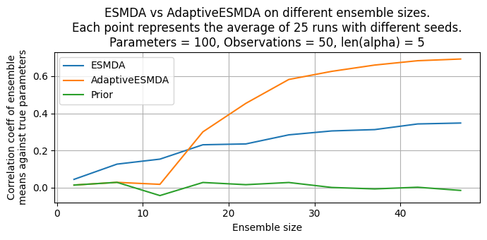
Run on several ensemble sizes and seeds

To get a more complete picture of how the number of realizations (ensemble size) affects the result, we loop over various ensemble sizes and compute posteriors. To capture average behavior and reduce the influence of sampling noise, we also loop over several seeds.

Recall that there are two sources of randomness in the result:

• The draw of prior realizations \(X \sim N(0, \sigma)\).

• The noise (given by the covariance argument) that ESMDA adds to the observations.

def corr_true(array):
    return sp.stats.pearsonr(x_true, array).statistic


ENSEMBLE_SIZES = list(range(2, 51, 5))
NUM_SEEDS = 25

# Store average correlation coefficients
ESMDA_corrs = []
AdaptiveESMDA_corrs = []
prior_corrs = []  # Baseline comparison - no update

# Loop over increasingly large ensemble sizes
for ensemble_size in ENSEMBLE_SIZES:
    # Posteriors means for this size
    ESMDA_means = []
    AdaptiveESMDA_means = []
    prior_means = []

    # Loop over seeds used in ESMDA/AdaptiveESMDA,
    # which determine the perturbations of the observations.
    for seed in range(NUM_SEEDS):
        # Prior
        X = get_prior(num_parameters, ensemble_size, prior_std)
        prior_means.append(np.mean(X, axis=1))

        # ================ ESMDA ==============
        smoother = ESMDA(
            covariance=covariance,
            observations=observations,
            alpha=5,
            seed=seed,
        )

        X_i = np.copy(X)
        for _ in range(smoother.num_assimilations()):
            smoother.prepare_assimilation(Y=g(X_i))
            X_i = smoother.assimilate_batch(X=X_i)

        ESMDA_means.append(np.mean(X_i, axis=1))

        # ============ AdaptiveESMDA ============
        adaptive_smoother = AdaptiveESMDA(
            covariance=covariance,
            observations=observations,
            seed=seed,
        )

        X_i = np.copy(X)

        for _ in range(adaptive_smoother.num_assimilations()):
            adaptive_smoother.prepare_assimilation(Y=g(X_i))
            X_i = adaptive_smoother.assimilate_batch(
                X=X_i, correlation_callback="three_over_sqrt_ensemble_members"
            )

        AdaptiveESMDA_means.append(np.mean(X_i, axis=1))

    # Collect results for all runs of this size
    ESMDA_corr = np.mean([corr_true(arr) for arr in ESMDA_means])
    AdaptiveESMDA_corr = np.mean([corr_true(arr) for arr in AdaptiveESMDA_means])
    prior_corr = np.mean([corr_true(arr) for arr in prior_means])

    # Add to respective lists
    ESMDA_corrs.append(ESMDA_corr)
    AdaptiveESMDA_corrs.append(AdaptiveESMDA_corr)
    prior_corrs.append(prior_corr)

# Create figure title with a lot of information
title = "ESMDA vs AdaptiveESMDA on different ensemble sizes.\n"
title += (
    f"Each point represents the average of {NUM_SEEDS} runs with different seeds.\n"
)
title += f"Parameters = {num_parameters}, Observations ="
title += f" {num_observations}, len(alpha) = {len(smoother.alpha)}"


# Create the figure
plt.figure(figsize=(7, 3.5))
plt.title(title)

plt.plot(ENSEMBLE_SIZES, ESMDA_corrs, label="ESMDA")
plt.plot(ENSEMBLE_SIZES, AdaptiveESMDA_corrs, label="AdaptiveESMDA")
plt.plot(ENSEMBLE_SIZES, prior_corrs, label="Prior")

plt.xlabel("Ensemble size")
plt.ylabel("Correlation coeff of ensemble\nmeans against true parameters")

plt.grid(True)
plt.legend()
plt.tight_layout()
plt.show()