# ruff: noqa: E402
# ruff: noqa: E501
Fitting a polynomial with Gaussian priors#
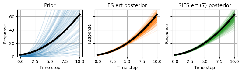
We fit a simple polynomial with Gaussian priors, which is an example of a Gauss-linear problem for which the results obtained using Subspace Iterative Ensemble Smoother (SIES) tend to those obtained using Ensemble Smoother (ES). This notebook illustrated this property.
import itertools

import numpy as np
import pandas as pd

np.set_printoptions(suppress=True)
rng = np.random.default_rng(12345)

import matplotlib.pyplot as plt

COLORS = list(plt.rcParams["axes.prop_cycle"].by_key()["color"])

plt.rcParams["figure.figsize"] = (6, 6)
plt.rcParams.update({"font.size": 10})
from ipywidgets import interact  # noqa  # isort:skip
import ipywidgets as widgets  # noqa  # isort:skip
from p_tqdm import p_map

import iterative_ensemble_smoother as ies
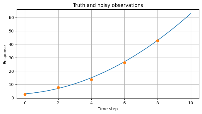
Define synthetic truth and use it to create noisy observations#
ensemble_size = 200


def poly(a, b, c, x):
    return a * x**2 + b * x + c


# True patameter values
a_t = 0.5
b_t = 1.0
c_t = 3.0

noise_scale = 0.1
x_observations = [0, 2, 4, 6, 8]
observations = [
    (
        rng.normal(loc=1, scale=noise_scale) * poly(a_t, b_t, c_t, x),
        noise_scale * poly(a_t, b_t, c_t, x),
        x,
    )
    for x in x_observations
]

d = pd.DataFrame(observations, columns=["value", "sd", "x"])
d = d.set_index("x")
num_obs = d.shape[0]

fig, ax = plt.subplots(figsize=(7, 4))
x_plot = np.linspace(0, 10, 2**8)
ax.set_title("Truth and noisy observations")
ax.set_xlabel("Time step")
ax.set_ylabel("Response")
ax.plot(x_plot, poly(a_t, b_t, c_t, x_plot))
ax.plot(d.index.get_level_values("x"), d.value.values, "o")
ax.grid()
fig.tight_layout()
plt.show()
Assume diagonal observation error covariance matrix and define perturbed observations#
R = np.diag(d.sd.values**2)

E = rng.multivariate_normal(mean=np.zeros(len(R)), cov=R, size=ensemble_size).T
assert E.shape == (num_obs, ensemble_size)

D = d.value.values.reshape(-1, 1) + E
Define Gaussian priors#
coeff_a = rng.standard_normal(size=ensemble_size)
coeff_b = rng.standard_normal(size=ensemble_size)
coeff_c = rng.standard_normal(size=ensemble_size)

X = np.vstack([coeff_a, coeff_b, coeff_c])
Run forward model in parallel#
fwd_runs = p_map(
    poly,
    coeff_a,
    coeff_b,
    coeff_c,
    [np.arange(max(x_observations) + 1)] * ensemble_size,
    desc="Running forward model.",
)
Pick responses where we have observations#
Y = np.array(
    [fwd_run[d.index.get_level_values("x").to_list()] for fwd_run in fwd_runs]
).T

assert Y.shape == (
    num_obs,
    ensemble_size,
), "Measured responses must be a matrix with dimensions (number of observations x number of realisations)"
Condition on observations to calculate posterior using both ES and SIES#
from iterative_ensemble_smoother.utils import steplength_exponential

X_ES_ert = X.copy()
Y_ES_ert = Y.copy()
smoother_es = ies.SIES(
    parameters=X_ES_ert,
    covariance=d.sd.values**2,
    observations=d.value.values,
    seed=42,
)
X_ES_ert = smoother_es.sies_iteration(Y_ES_ert, step_length=1.0)


X_IES_ert = X.copy()
Y_IES_ert = Y.copy()
smoother_ies = ies.SIES(
    parameters=X_IES_ert,
    covariance=d.sd.values**2,
    observations=d.value.values,
    seed=42,
)
n_ies_iter = 7
for i in range(n_ies_iter):

    step_length = steplength_exponential(i + 1)
    X_IES_ert = smoother_ies.sies_iteration(Y_IES_ert, step_length=step_length)

    _coeff_a, _coeff_b, _coeff_c = X_IES_ert

    _fwd_runs = p_map(
        poly,
        _coeff_a,
        _coeff_b,
        _coeff_c,
        [np.arange(max(x_observations) + 1)] * ensemble_size,
        desc=f"SIES ert iteration {i}",
    )

    Y_IES_ert = np.array(
        [fwd_run[d.index.get_level_values("x").to_list()] for fwd_run in _fwd_runs]
    ).T
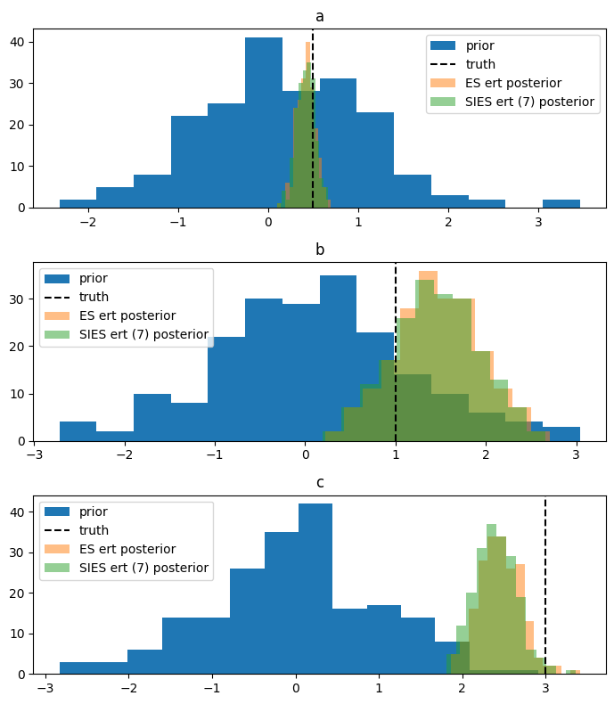
Plots to compare results#
def plot_posterior(ax, posterior, method):
    for i, param in enumerate("abc"):
        ax[i].set_title(param)
        ax[i].hist(posterior[i, :], label=f"{method} posterior", alpha=0.5, bins="fd")
        ax[i].legend()

    fig.tight_layout()
    return ax


fig, ax = plt.subplots(nrows=3, figsize=(7, 8))

for i in range(3):
    ax[i].hist(X[i, :], label="prior", bins="fd")

ax[0].axvline(a_t, color="k", linestyle="--", label="truth")
ax[1].axvline(b_t, color="k", linestyle="--", label="truth")
ax[2].axvline(c_t, color="k", linestyle="--", label="truth")

plot_posterior(ax, X_ES_ert, method="ES ert")
_ = plot_posterior(ax, X_IES_ert, method=f"SIES ert ({n_ies_iter})")
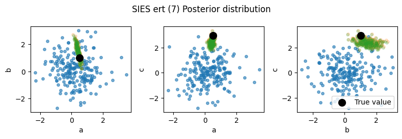
fig, axes = plt.subplots(1, 3, figsize=(8, 2.75))
axes = axes.ravel()
labels = "abc"
true_parameters = [a_t, b_t, c_t]

fig.suptitle(f"SIES ert ({n_ies_iter}) Posterior distribution")
for k, (i, j) in enumerate(itertools.combinations([0, 1, 2], 2)):
    axes[k].scatter(X[i, :], X[j, :], s=15, alpha=0.6)
    axes[k].scatter(X_ES_ert[i, :], X_ES_ert[j, :], s=15, alpha=0.2)
    axes[k].scatter(X_IES_ert[i, :], X_IES_ert[j, :], s=15, alpha=0.2)
    axes[k].scatter(
        [true_parameters[i]],
        [true_parameters[j]],
        color="black",
        s=100,
        label="True value",
    )
    axes[k].set_xlabel(labels[i])
    axes[k].set_ylabel(labels[j])


axes[k].legend()
fig.tight_layout()
plt.show()
fig, (ax1, ax2, ax3) = plt.subplots(1, 3, figsize=(8, 2.5), sharex=True, sharey=True)
x_plot = np.linspace(0, 10, 2**8)

# Plot the prior
ax1.set_title("Prior")
ax1.plot(x_plot, poly(a_t, b_t, c_t, x_plot), zorder=10, lw=4, color="black")
for parameter_prior in X.T:
    ax1.plot(
        x_plot, poly(*parameter_prior, x_plot), color=COLORS[0], alpha=0.1, zorder=5
    )

# Plot the posterior
ax2.set_title("ES ert posterior")
ax2.plot(x_plot, poly(a_t, b_t, c_t, x_plot), zorder=10, lw=4, color="black")
for parameter_posterior in X_ES_ert.T:
    ax2.plot(
        x_plot, poly(*parameter_posterior, x_plot), alpha=0.1, zorder=5, color=COLORS[1]
    )

# Plot the posterior
ax3.set_title(f"SIES ert ({n_ies_iter}) posterior")
ax3.plot(x_plot, poly(a_t, b_t, c_t, x_plot), zorder=10, lw=4, color="black")
for parameter_posterior in X_IES_ert.T:
    ax3.plot(
        x_plot, poly(*parameter_posterior, x_plot), alpha=0.1, zorder=5, color=COLORS[2]
    )

# Common axes setup
for ax in [ax1, ax2, ax3]:
    ax.set_ylim([0, 70])
    ax.set_xlabel("Time step")
    ax.set_ylabel("Response")
    ax.grid(zorder=0)

fig.tight_layout()
plt.show()